PDEOpNet
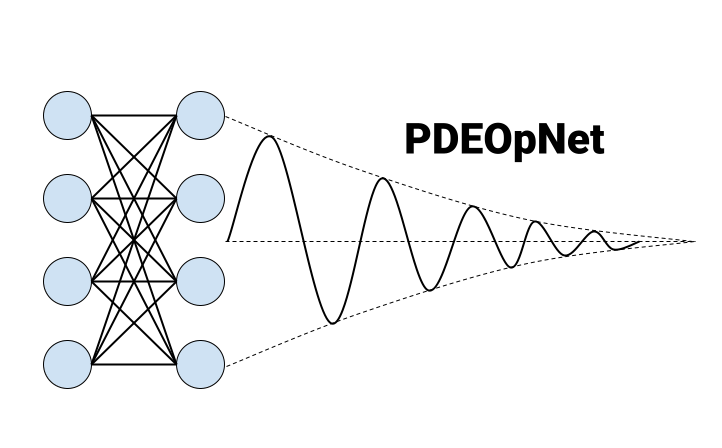
PDEOpNet - EECS 351
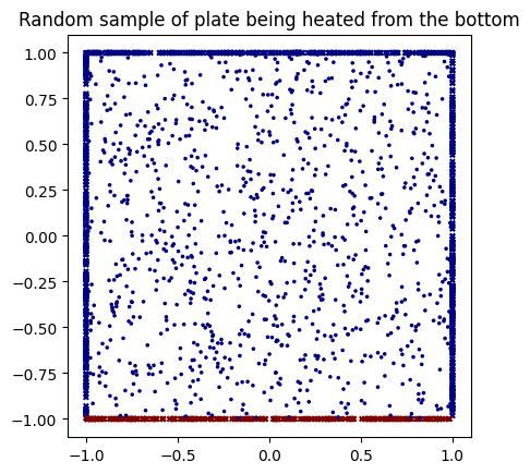
Data
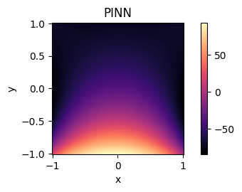
PINN
Interestingly, we did not have to collect nor generate any data for the physics-informed neural network. Instead, we just enforced constant Dirichlet boundary conditions along the square’s edges (representing a metal plate), and then randomly sampled various collocation points along the plate’s surface where we enforced the physics-informed loss term of our objective function. Note that all the non-boundary points had zero initial conditions. An advantage of PINNs, as we’ve discussed, is that they require less training data due to the physics-informed loss guiding the solution approximation.
To be more precise, we trained on a square with x and y both bounded by -1 below and 1 above, and sampled 2000 collocation points at random non-boundary points within said square. All non-boundary points were initialized with zero initial conditions, whereas the lower side was initialized with value 1 (hot), and the other three sides with value -1 (cold); note that these values, being the Dirichlet boundary conditions, were then held constant throughout the training process. Here is an example input and output to the PINN:
Fourier PINN
The Fourier PINN was very similar. Notice that in the first cell of the data preparation section, you can change the parameters for number of (collocation) points across the plate, the border coordinates of the square (e.g., [0, 1] would create a unit square), and the upper and lower bounds of the temperature values. This allows us the ability to programmatically build new simulations with different areas, greater or smaller number of points, and varying temperature ranges, to see how well our model generalizes to new scenarios by comparing the different performances.
Neural Operator
Since neural operators are a continuous function-to-function mapping, and images are essentially functions of two-dimensional space (x and y), we can think of the neural operator as a continuous image-to-image mapping. Hence, we had images (of the same dimension) as input and output. Specifically, the images we generated are 64x64, with the heat intensity values at each pixel ranging from continuous values between -1 and 1. We generated this data by modifying the following code, which solves the Laplace equation (which is just the steady state heat equation). We iterated it 2000 times to generate 2000 training pairs of images. The inputs were generated with (uniformly) randomly selected boundary conditions between -1 and 1, and zero initial conditions for all non-boundary points on the plate surface. In each iteration, we then solved the Laplace equation to get the steady state heat solution for our random initial state, and this image would be the corresponding output of the training pair. We found that solving for the steady state outputs did not take very long (especially compared to using Finite-Difference or Finite-Element methods, which would be necessary to see the time-evolution or non-steady state solutions), so most of the time was spent uploading them (as saved .npy files) to Google Drive. Then, our group members could access the training pairs using the Colab files.
Before we decided to generate our own (synthetic) data, we found a dataset online which was generated for a paper which uses different machine learning techniques to solve essentially the same problem as us; finding the steady state solution to the heat equation, in their case for the purpose of studying heat conduction transfer. However, their dataset had varying geometries (e.g., rectangles, triangles, other shapes); this made sense for them as they used a convolutional neural network, and convolutional filters are translationally-invariant, meaning the network could better adapt to different plate geometries. Based on our understanding of neural operators (and PINNs), however, we didn’t think our network(s) would generalize well to this training scheme, as they probably wouldn’t capture wider-range space dependencies in the solution domain without some modification. A recent paper by Zongyi Li (one of the original authors of neural operators) et al. proposes a geometry-informed neural operator (GINO) that uses both graph and Fourier architecture to account for varying geometries. At a high level, it maps irregular grids to regular latent grids where the FNO can be applied. This could definitely be a future extension to our project given more time and resources.