PDEOpNet
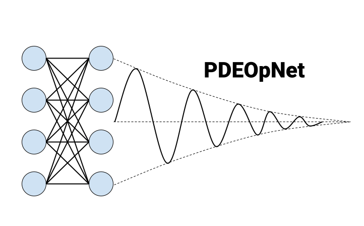
PDEOpNet - EECS 351
Project Progress Report (17 November 2023)
This page is the Project Progress Report for 17 November 2023. This page will discuss the state of the project as of that date. We will begin by describing the data used for our project and how it was attained. We will then present three plots of our data to help visualize key aspects of our progress. We will describe more generally what work we have done so far, and create a plan for the coming weeks until the project due date. Finally, we will provide a brief reflection on what we have learned so far.
Data
As our model is solving differential equations, our data are samples of the systems defined by the differential equation. For our first PINN model, we are specifically attempting to model the heat equation, thus our data can be thought of as the initial and final states of a thermodynamic system. In our case, we are specifically training on a 2-dimensional model of heat transfer. Thus, for \(N\) samples in space we have \(d=3\) dimensions representing the \(xy\) location and initial temperature, \(T\) of the point sample. Thus, our input data, \(D_{in}\) can be viewed as a second-degree tensor:
\[D_{in} = \begin{bmatrix} x_0 & y_0 & T_0 \\ x_1 & y_1 & T_1 \\ ... & ... & ... \\ x_N & y_N & T_N \end{bmatrix}\]As we are attemping to solve the heat equation, our labels, or the targets for our prediction, are simply the end thermodynamic states of each point sample. However, we do this differently than a simple MSE loss – we treat the boundaries as constant temperature, and impose a different loss term for the samples not on the boundary of the plate (see Visualizations for a better understanding of boundary vs interior points). Because we only compute MSE loss with respect to constant-temperature boundaries, we can actually use the input data to compute our loss. Thus, we only need one set of points to estimate the solution to the PDE!
For further information regarding how this data was generated, please refer to Work Completed below.
Visualizations
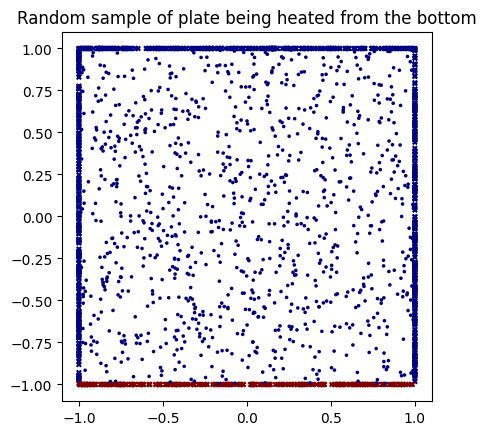
These figures depict three key states of data in our project. The first figure depicts the input data to our model, a set of random point samples in a 2-dimensional space where heat is applied by a plate at \(y=-1\). In this initial state, the points in space start with no heat, and only the boundary points along \(y=-1\) are heated. We generated this by randomly sampling an evenly-distributed set of points in \(xy\) space, and enforcing initial heat along the bottom points.
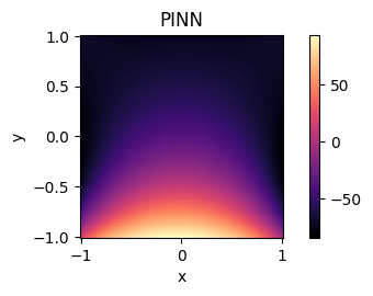
The next two figures depict the final state of our thermodynamic system under varied differential loss regularizations. The first figure depicts the final state of the thermodynamic system when our PINN is regularized to model the standard heat equation:
\[\frac{\partial u}{\partial t} = \Delta u\]As shown in the figure, heat, depicted as brighter pixels, radiates evenly in space. The heat decreases radially from the heated plate.
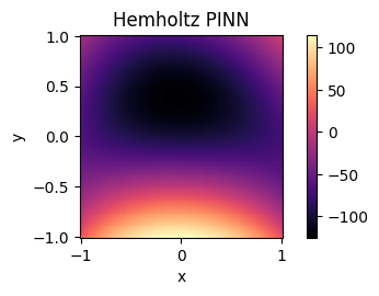
The second figure depicts the final state of the thermodynamic system when our PINN is regularized to model the Helmholtz equation. The Helmholtz equation is only different in one term from the standard heat equation, and captures the eigenvalue problem for the Laplace operator:
\[\nabla^2 f = -k^2 f\]Interestingly, introducing this regularization causes the heat to radiate more consistently along the edges. The heat depicts a similar diffusion around the space of the hot plate, but the edges and corners of the space boundry show higher heat.
Work Completed
Prior to this week, our team spent a majority of our time reading the current literature surrounding PDEs, PINNs, and neural operators. Due to the largely conceptual nature of this field, we had to consult countless resources including published literature, articles, recorded lectures, and more to fully understand the space. We found that, in many ways, this is still a very cutting-edge disclipline, with several milestone pieces having been published in recent months. As such, this rapidly-developing field necessarily lends itself to new ideas and creativity in ways that more established fields of study may not.
Given the nebulus and quickly-changing nature of our topic, we decided it was imperative to identify key deliverables for our project so we could avoid getting lost in the flux of new work. With this in mind, this week we solidified our final plans for the structure of our project, and delegated necessary tasks to each member. We began by establishing the key goals enumerated on the cover page of this website. We seek to:
- Develop a PINN model to solve important families of PDEs
- Modify this model to transform data and compare performance across multiple bases of representation
- Attempt to generalize our model as a neural operator, allowing us to not just solve PDEs numerically, but capture the functional structure of a PDE solution in our network
With these goals in mind, we then delegated and began necessary tasks. Of primary importance was creating training and testing data, developing the first baseline PINN model, and researching neural operators.
To create training data, we simply sampled many points in the unit square, and imposed a “hot” side as the initial heat source. We were amazed how PINNs allowed us to simply tell the network some initial conditions, some constant conditions, and impose some PDE-derived facts about the estimated solution. This allowed us to compute our own input dataset numerically, and let the imposed regularization term guide the network in training. We defined an initial state \(D_{in}\) in the form described above in Data, and used this same data to compute loss during model training. We completed this in Python using TensorFlow and Numpy GPU operations for rapid calculation.
We then began defining our first PINN model using Keras. This model is a Multi-Layer Perceptron (MLP), meaning that the network is fully-connected. We found that this architecture worked well to capture the dynamics of the heat equation, and was consistent with the fact that a closed-form solution exists.
Next, we tried to see how extendable our initial heat-equation implementation was to other types of equations. We turned to the Helmholtz equation \((\Delta + k^2)f = 0\), a one-term deviation from the heat equation as the next PDE. Unsurprisingly, all it took was to update the PDE regularization term during network training. It’s clear that the Helmholtz solution has more wave-like periodic properties in our visualization, which matches the applications of the equation generally.
Finally, we read several papers on neural operators to begin to understand how we can research and implement these in our project. Neural operators allow for discretization-invariant function approximation, a defining characteristic that could speed up partial differential equation system simulation more 1000x over slow, traditional numerical methods. Notably, they are also much more general than PINNs, which are restricted to the initial conditions they are trained on.
Plan for Completion
The next steps for our project are severalfold, however they are largely defined by 2 paths that will be worked on in parallel, by 2 members each.
- Complete analysis of multiple-basis representation
- Create PINN with Fourier transform layer and compare performance
- Create PINN with Laplace transform layer and compare performance
- *Create PINN with z-transform layer and compare performance (possible extension)
- Recommend best basis for representing point samples for our PINN
- Investigate and create neural operator model to compare performance
- Implement neural operator model and test viability on several PDE families
- Compare performance to above PINN models
- Discuss costs and benefits regarding trainig time, accuracy, stability, and generalizability
Upon completion of the above tasks, we will be prepared to present a review of the many models and methods that are currently being researched in this field. Because of the rapidly-changing nature of PINN, PDE, and neural operator research, we believe that providing a comparative study such as this will provide a necessary guidepost for researchers and observers alike. Beyond providing a review of the field, we will also be introducting new approaches that are unexplored in literature such as the z-transform PINN model, typifing our intent to not only understand, but to contribute to this field.
Reflections on Learning
We have learned countless new theories and skills while working on this project. Among the most interesting to us have been some key characteristics of machine learning models.
While doing preliminary research and reading for this project, we were surprised to learn that the power of neural networks can extend to a decidedly “continuous” domain like differential equations. This is explained by a concept called the Universal Approximation Theorem. First explored by Kurt Hornik, Maxwell Stinchcombe, and Halbert White at the Technische Universität Wien and University of California, San Diego in 1989, the universal approximation theorem states that feedforward neural networks (FNN) can effectively approximate any function from one finite dimension space to another. Although this would require an extremely large number of hidden layers and activations to be exhibited in totality, this means that, for a given degree of accuracy, we can reasonably model any function with the correct model architecture. This was an extremely interesting conclusion for our group, and helped us understand why FNNs could be used to approximate solutions to PDEs. More generally, it also speaks to the power and significance of machine learning as a field. By embracing these data-driven methods of research and discovery, even the most intractable systems can be understood.
We also learned more about regularization in machine learning and how that can be leveraged to guide the fit for a model. In machine learning, regularization broadly refers to techniques that tune models during training. This is commonly done by introducting terms in the loss function for a model, thus incentivizing or decentivizing certain behavior. Our group had previously seen this in regularization techniques like sparsity regularization, which incentivizes sparse model weights in an attempt to make training less intensive, more compressed, and sometimes even more interpretable. In the context of this project, our group learned about using regularization to fit a model to a certain functional relationship. In this case, we want to enforce that our network, approximating the function \(f\) will adhere to the form of a partial differential equation, or, for the heat equation in a k-dimensional space:
\[\Delta f = \sum_{i=1}^k\frac{\partial^2 f}{\partial x_i^2} = 0\]We can enforce this structure in our network through our loss function, which will penalize approximations that deviate from this form. This is an extremely powerful technique, and is the physics concept that defines a physics-informed neural network.