Results

Below, we will present and discuss our results for the three major model architectures that were explained in methods. Because each architecture has its own strengths and weaknesses, our results suggest that certain methods are best suited for certain scenarios. By exploring these results and drawing more general conclusions, we help to clarify the variable effectiveness and future use cases of each of these model architectures.

PINN

We trained and tested our PINN model on three different scenarios. In all three cases, the learning rate was held constant at 5e-4. A table describing those three scenarios is below:

Simulation	num_sample_points	border_coordinates	temp_range	epochs	k
1	2000	[-1,1]	[-1,1]	3000	1
2	2000	[-1,1]	[-1,1]	2000	2
3	8000	[-5,5]	[-3,3]	2000	2

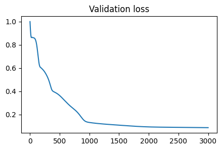
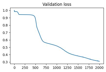
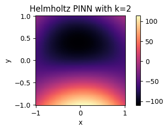
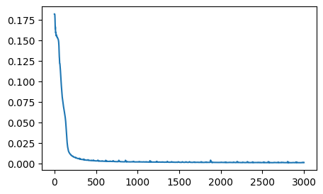
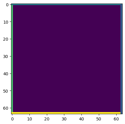
The train and test results from simulation 1 are below:

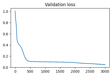
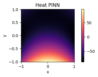
The top plot demonstrates the validation loss over our 3000 epochs of training for simulation 1. As we can see it succesfully converges, suggesting a strong model fit was achieved. The bottom plot depicts the final state of the hot plate system. We have successfully captured the radiant heat eminating from the bottom, hot edge of the plate, suggesting we have accurately modeled the dynamics of our system. Importantly, the edges have maintained their constant temperature, as enforced by our boundary loss, and the sample points distributed throughout the plate now respect the heat equation.

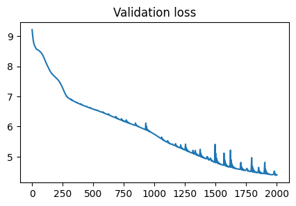
The train and test results from simulation 2 are below:

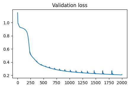
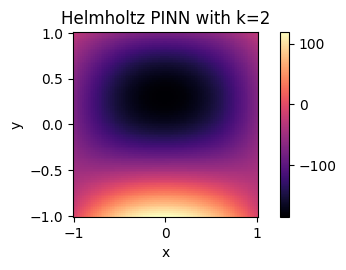
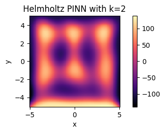
Similarly, the validation loss depicted in the top plot suggests convergence over our training time for simulation 2. Notably there are slight spikes in the validation loss once the model approaches convergence. While it is difficult to pinpoint the exact reason for this in such a deep model, we believe it may appear as an artifact of training, where gradients briefly “explode” for certain points. For example, these spikes could occur between training epochs, resulting in a significant shift in gradient, and thus loss, as the model moves from propagating the last point of the previous epoch to the first point of the new epoch. Importantly, the bottom plot’s depiction of the final state of the Helmholtz-modified hot plate system is consistent with our expected results, suggesting we have again accurately modeled our system.

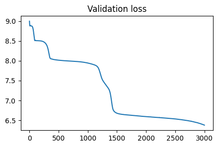
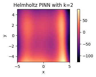
The train and test results from simulation 3 are below:

Again, the validation loss in the top plot suggests that we have achieved convergence over our training time for simulation 3. However, we see an odd, periodic banding effect across the plate. We believe this is likely due to model underfitting, a limitation of the basic PINN architecture. Rather than spreading evenly throughout the space, we see a periodic shape that, while sourcing from the bottom of the plate, is not wholly accurate to the expected output of the Helmholtz system.

Overall, our PINN has provided solid output for our heat and Helmholtz scenarios. While it has some fitting issues with a larger system region and Helmholtz constant, it overall performs well for being a relatively simple architecture. Thus, we conclude that the PINN is well-suited for simple systems where initial conditions are consistent and there are not too many high-frequency elements in the system. While the model must be re-trained for different system initial conditions, once trained it can provide accurate and consistent outputs at smaller scales.

Fourier PINN

For direct comparison with our PINN, we trained and tested our FPINN model on the same three different scenarios. In all three cases, the learning rate was held constant at 5e-4. Note that simulation 3 for the FPINN was trained over 3000 epochs versus the 2000 epochs trained for simulation 3 for the PINN.

Simulation	num_sample_points	border_coordinates	temp_range	epochs	k
1	2000	[-1,1]	[-1,1]	3000	1
2	2000	[-1,1]	[-1,1]	2000	2
3	8000	[-5,5]	[-3,3]	3000	2

The train and test results from simulation 1 are below:

Just as with the PINN implementation for simulation 1, we see a similar level and rate of convergence in the top plot, which shows the validation loss over the 3000 epochs of training for our FPINN. The bottom plot again depicts the final state of the hot plate system, which captures the expected radiant heat dynamics, and is consistent with the PINN model output.

The train and test results from simulation 2 are below:

Again, the validation loss converges, after a slight plateau for the first several hundred epochs. While this could look like convergence if we did not train past 500 epochs, this suggests that in this region we had not yet fit our model fully. Thus, it was important that we continued to expand the number of training epochs to where we steady decline as shown in the plot above. Again, the final state is consistent with the Helmholtz system and mirror the output of the PINN on scenario 2.

The train and test results from simulation 3 are below:

The valiation loss converges after demonstrating a slight plateau effect, much as occurred in simulation 2. Yet again, we trained past this plateau to the full 3000 epochs as set in our testing strategy. The system appears to reach a more consistent state than our PINN for simulation 3. We see there is a more progressive gradient in “heat” over the plate, and there are no significant oscillatory effects as with the PINN. This suggests that the FPINN can more accurately capture and interpret the high-frequency dynamics of the Helmholtz equation.

While suffering from the same initial conditions limitation as the PINN, the FPINN appears to perform well at capturing and representing high-frequency system dynamics. In the Helmholtz equation model, it accurately captures and “smoothes” out the high-frequency terms in the system which arise from the squared constant in the equation. Again, the FPINN is trained dependent on initial conditions and would need to be retrained for structurally-different initial conditions, but the emphasis of high-frequency components in the model allows us to achieve consistently competitive results despite a smaller architecture.

FNO

For our FNO implementation, we trained and tested a single scenario over 3000 epochs.

The train and test results from this simulation are below:

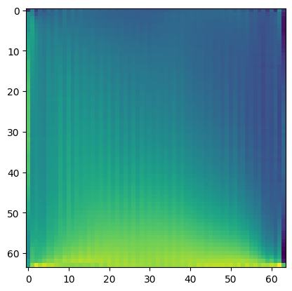
Training is yet again stable, and converges after approximately the first 1000 epochs. Importantly, the input for this simulation is effectively arbitrary, meaning the model has no knowledge of initial conditions. This is demonstrated in the second plot above, which shows the variable heating on each edge of the hot plate. Unlike the PINN and FPINN, this model effectively captures the total system dynamics of the heat equation, not just the system dynamics of a specific scenario and initial condition to the heat equation. We can see that in the final plot above, we have heat distributed evenly across the plate, with a gradient proportional to each edge’s initial temperature.

Due to the more general nature of the model, it also exhibits a property known as mesh invariance. If every pixel covers some 2d region of the plane, the representative field of each pixel changes as we scale our plot up or down. For example in a \((64 \times 64)\) plane, each pixel covers “more” than a more granular \((128 \times 128)\) plane. Because of the FNO’s ability to handle arbitrary initial conditions, it is robust to this mesh invariance as well. No matter the granularity of the pixels that are sampling and representing the underlying continuous system, the model will disperse correctly and apply the dynamics of learned differential equation.

This model succeeds at combining the strengths of both previous models, while additionally being robust to changing initial conditions. This is especially important for real-world applications, as initial conditions will change wildly in most experimental and applied settings.

Conclusions

While all models have their strengths and weaknesses, the three models differ largely in their complexity, ability to capture high-frequency dynamics, and robustness to initial system conditions. The PINN is a simple model, but is not particularly strong at capturing high-frequency system dynamics, and is fully dependent on system initial conditions. The FPINN is similarly simple and dependent on initial conditions, but can capture high-frequency dynamics very well. Finally the FNO, though complex, is the most generalizable, allowing it to capture high-frequency dynamics and be robust to system initial conditions. Thus, if enough compute resources are available, we suggest that the Fourier Neural Operator model is the most for learning the dynamics of partial differential equations. Although it can be difficult to train, its generalizability with continued focus on frequency-domain learning, allows it to most accurately, and most consistently, model differential equations.

DSP Topics

To achieve the results above, we had to rely heavily on several key topics from class. We employed principles of the Fourier transform and multiple basis representation for both the FPINN and FNO. We used these in a particularly applied context as we used torch.fft.fft and torch.fft.ifft to perform Fast Fourier Transforms as discussed in class. This was necessary to allow our model to quickly train and test in both spatial and frequency domains. Additionally, we also used and built upon the core principles of machine learning that we learned in class. The foundations of MLPs, neural networks, activation functions, and more were a central part of this work.

We used several tools from beyond class. For example, we learned and used PyTorch to create our machine learning models. We also learned about interesting system properties that, while much like those for signals, are more particular to machine learning for partial differential equations such as mesh invariance, initial condition invariance, and the Universal Approximation Theorem.