Methods

On this page we will discuss the major machine learning methods employed to analyze partial differential equations. The three architectures that we analyze represent a progression in difficulty. In architecture, implementation, and analysis, each successive architecture becomes more complex, but leverages key techniques to better capture, characterize, and represent our desired systems.

The first architecture is a simple Physics-Informed Neural Network (PINN). The core of this architecture is a multi-layer perceptron (MLP) that learns system final conditions based on initial conditions.

We follow this with the more complicated Fourier Physics-Informed Neural Network (FPINN), which leverages a Fourier learning layer to learn in multiple bases and capture more nuanced dynamics of the system.

Finally, we conclude with a Physics-Informed Neural Operator (PINO) which unites techniques from the FPINN and a new training cycle to capture generalizable differential operators.

More detail on all three models is presented below. By developing these three models, we have a strong baseline to compare and discuss model shortcomings and effectiveness.

PINN

The Physics-Informed Nerual Network (PINN) was implemented in PyTorch, based on the original paper and corresponding TensorFlow implementation from Raissi et al. at Brown University and the University of Pennsylvania. In addition to redeveloping this architecture in PyTorch, our implementation introduced several novel features, including a new way to customize training scenarios, a modified model architecture, and new loss functions. The training scenario customization is discussed in full on our data page.

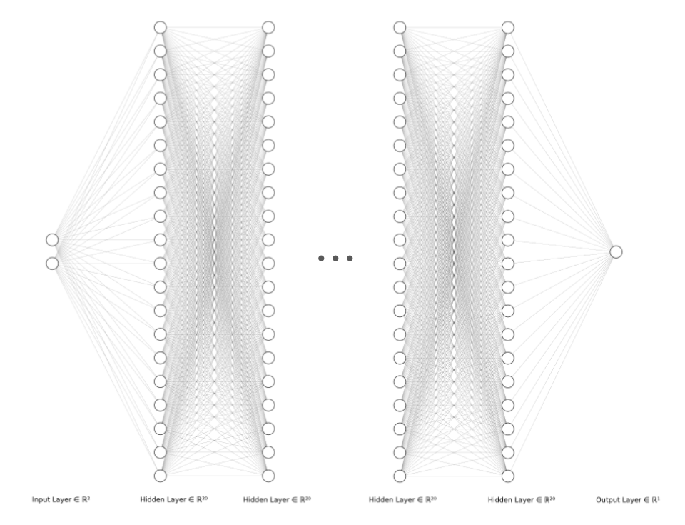
The PINN architecture is a multi-layer perceptron (MLP), meaning that all activations are fully connected. At a high level, this MLP is responsible for transforming an \((x,y)\) coordinate to a predicted temperature. Each fully-connected layer is followed by a tanh activation function, which maps each activation to the range \(\alpha \in (-1, 1)\). The architecture contains seven fully-connected layers, each with 20 activations. We created a diagram to depict our architecture visually below. As seen in the diagram, there are two input nodes, one for each of \((x,y)\), seven fully-connected layers, truncated for space, and the output layer, a scalar temperature prediction node.

To train our model, we used two loss terms to enforce boundary conditions and differential loss. Our differential loss was altered from the original paper and implementation, seeking to solve the Helmholtz equation in addition to the heat equation. The two loss functions are below, where \(u\) is the scalar output of the network, \(k\) is the Helmholtz constant which is chosen per-system, \(t\) and \(\hat{t}\) are the ground truth and predicted boundary temperatures, and \((x,y)\) represent a collocation point in space.

\[\mathcal{L}_{boundary} = \text{mean}((t - \hat{t})^{2})\] \[\mathcal{L}_{PDE} = \text{mean}((\frac{\partial^2 u}{\partial x} + \frac{\partial^2 u}{\partial y} + k^2 \cdot u)^2)\] \[\mathcal{L}_{total} = \mathcal{L}_{boundary} + \mathcal{L}_{PDE}\]

The boundary loss enforces the Dirichlet boundary condition. In this case we require that the temperature of all boundary points must stay the same between the initial state and final state, and penalize any model that changes the temperature of boundary points. The PDE loss requires that the collocation points, or the sample of points throughout the plate, observe the gradients of our differential equation. In this case, we use the Helmholtz equation, penalizing any model whose collocation points do not follow this differential equation.

Fourier PINN

The Fourier Physics-Informed Neural Network (FPINN) was similarly implemented in PyTorch, built off the core of the PINN. The major new feature of this architecture was a novel Fourer layer, inspired by the work of Li et al. at Caltech. This layer, which seeks to capture and learn from frequency information alongside spatial information, allows the FPINN to more effectively learn systems with high-frequency components.

As established by Rahaman et al., neural networks have a “spectral bias” towards smoothness and low frequencies. Because of this, it can often be difficult to generalize solutions that have strong, high-frequency components. To rectify this, we consulted several potential solutions to pay closer attention to these frequency components.

Our first approach was with an operation known as Fourier upsampling. As initially discussed by Tancik et al., this Fourier upsampling would essentially allow the network to learn “high frequency functions in low dimensional domains”, thus prompting our architecture to pay closer attention to, and learn from, high-frequency information. The two suggested upsampling approaches below are applied to the inputs, and passed through the rest of the network. In our case, \(\mathbf{v}\) is simply the \((x,y)\) coordinate of each collocation point. For the Gaussian Fourier upsampling \(\mathbf{B} \in \mathbb{R}^{m \times d}\) is sampled from \(\mathcal{N}(0, \sigma^2)\) where we selected unit variance.

\[\textbf{Basic:} \: \gamma(\mathbf{v}) = \left[\cos(2\pi \mathbf{v} \mu), \sin(2\pi \mathbf{v} \mu)\right]^{T}\] \[\textbf{Gaussian:} \: \gamma(\mathbf{v}) = \left[\cos(2\pi \mathbf{B} \mathbf{v} \mu), \sin(2\pi \mathbf{B} \mathbf{v} \mu)\right]^{T}\]

After building custom PyTorch layers to perform both methods of Fourier upsampling, we were getting inconsistent results. These are discussed in more detail in our results section, however these failures guided us to our second approach, the Fourier weighting layer.

Our second and final approach was to use a Fourier weighting layer with bypass. This layer learns on spatial and frequency representations simultaneously, allowing the network to use key information from both and variably weight either representation as needed. The diagram below comes from the previously discussed paper by Li et al.:

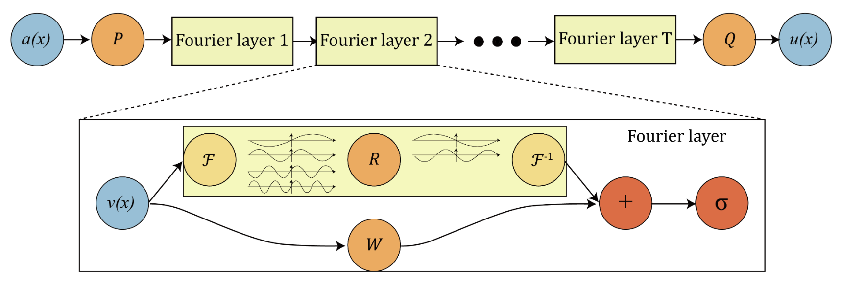
As can be seen in the diagram, each Fourier layer works on two representations simultaneously. The input is transformed with a Fast-Fourier Transform (FFT) into the frequency domain, scaled and shifted by weight and bias matrices, then transformed back to the spatial domain with the Inverse Fast-Fourier Transform (IFFT). The spatial input is also scaled and shifted by separate weight and bias matrices. This allows the network to learn in both bases, capturing and learning important information from both representations. The custom PyTorch Fourier layer that we developed is below:

class FourierLayer(nn.Module):
  def __init__(self, size_in, size_out):
    super().__init__()
    self.size_in, self.size_out = size_in, size_out

    w = torch.zeros([size_out, size_in], dtype=torch.float32, device=torch.device('cuda'))
    self.w = nn.Parameter(w)
    wb = torch.zeros([size_out], dtype=torch.float32, device=torch.device('cuda'))
    self.wb = nn.Parameter(wb)

    r = torch.zeros([size_out, size_in], dtype=torch.cfloat, device=torch.device('cuda'))
    self.r = nn.Parameter(r)
    rb = torch.zeros([size_out], dtype=torch.cfloat, device=torch.device('cuda'))
    self.rb = nn.Parameter(rb)

  def forward(self, x):
    fcoeff = torch.fft.fft(x)
    ftransform = torch.matmul(fcoeff, self.r.T) + self.rb
    fmat = torch.fft.ifft(ftransform)
    skip = torch.matmul(x, self.w.T) + self.wb

    return fmat.real + skip

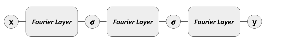
With this layer completed, we then built out the rest of our architecture. Far simpler than the PINN, this model only requires three Fourier hidden layers. All but the last layer are followed by a sigmoid activation function. Just as with the PINN, this model transforms an \((x,y)\) coordinate to a predicted temperature. Our visualizaton of the FPINN architecture is below:

To train the model, we used the same \(\mathcal{L}_{boundary}\), \(\mathcal{L}_{PDE}\), and \(\mathcal{L}_{total}\) as above. This makes sense as we are not changing our training objective, we are simply prompting our FPINN to pay closer attention to different features than the original PINN.

FNO

The Fourier Neural Operator is a neural network trained to learn the differential operator that solves a PDE. This is a natural next step following PINNs and FPINNs, because it allows us to set arbitrary initial conditions. Neural operators are designed to map between function spaces; specifically in our case, the input of the network is a function (the initial state) and the output is also a function (the final steady state). This makes it so that the neural operator is discretization-invariant; even though you’re training on finite, sampled data, since you’re learning functions, you still get a continuous function output, so you can discretize that output (as well as the input you’re training on) however you want. This is a great advantage of using neural operators to solve PDEs.

This is a very similar architecture to the Fourier layers we described for the FPINN. The difference here is that we are taking whole images through the network (thinking of images as functions of two-dimensional space); hence, the inputs and outputs are both images representing the initial and steady states, respectively. We begin by using rfft2 to exploit the symmetry of the real signals in the frequency domain (essentially, we can discard half of the FFT, so this is faster than using a full FFT). Then, we perform a linear transformation in the Fourier domain using a square matrix, so it left-multiplies the FFT coefficients and preserves the image shape. Then, we inverse rfft2 back to the spatial domain. We also have a skip connection that meets up here, just as in the Fourier PINNs (refer to the previous diagram), and said skip allows us to preserve high-frequency information in the input that may be lost in the Fourier path.

An extension of the FNO that relates to our PINN, although we did not have the time for it, are Physics-Informed Neural Operators (PINOs). These networks are neural operators, learning the differential solution operator the PDE, but instead of just being an FNO architecture, we also introduce the physics-informed loss term, depending on what our dynamical system is. Again, the input and output of the network are both functions. The difficulty with physically informing with image inputs is that there are no longer x and y coordinates to differentiate w.r.t. To do this, the official PINO implementation recasts the image-to-image problem as working with 3xN matrices (x, y, f(x,y)) in one dimension, and (size(matrix))^2 in the other dimension. This makes the physics informing possible, but we see that the solution operator we learned is good regardless.